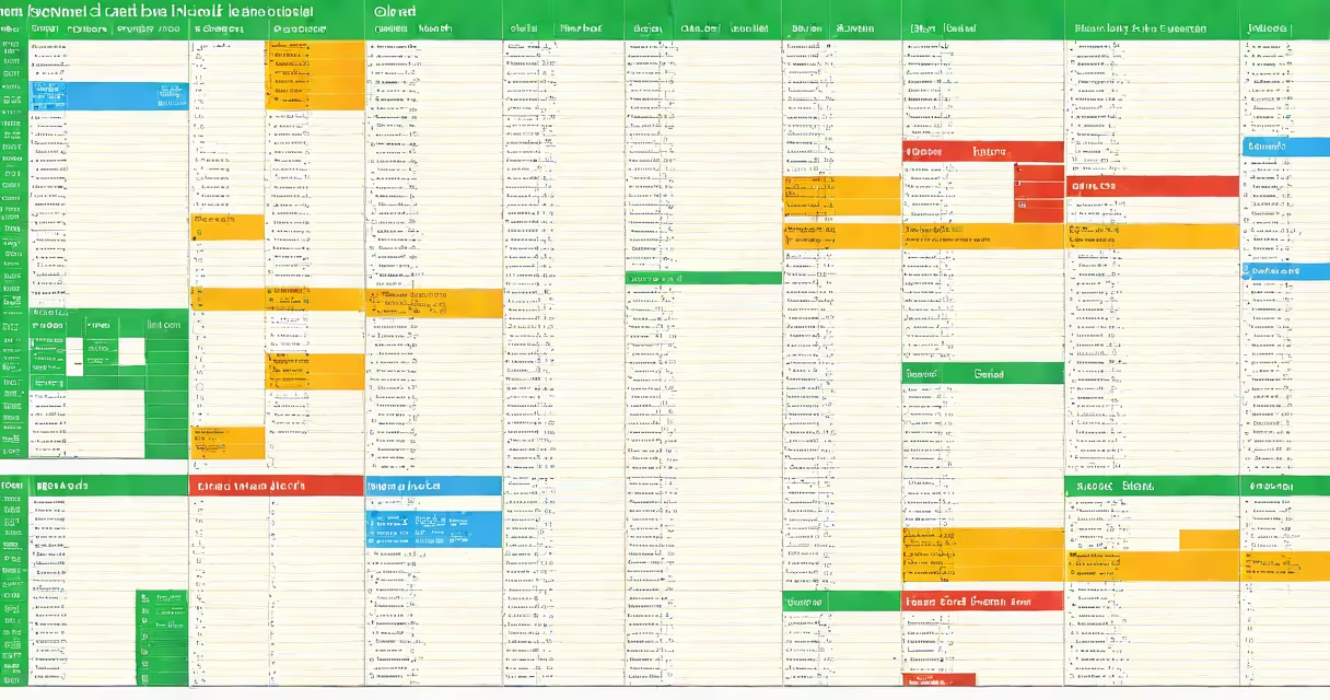
Formatting cells in Excel means changing their appearance and behavior using colors, fonts, borders, and specific number formats. This improves data organization and readability.
Excel applies formatting to cells based on their contents. For example, dates appear differently than numbers. You can override default formats to standardize data presentation.
Formatting doesn't affect calculations but makes data easier to interpret. For instance, applying red font to negative numbers highlights them visually.
| Format Type | Description | Example |
|---|---|---|
| Number Format | Controls how numbers display (decimal places, currency symbols) | $1,234.56 |
| Font Style | Changes text appearance (bold, italic, color) | Important Text |
| Alignment | Adjusts text position within cells (left, center, right) | Centered Text |
| Border | Adds lines around cells or groups | Thick black border |
| Fill Color | Changes cell background color | Light blue fill |
Use formatting to distinguish between data types (e.g., red for negatives, green for positives). It also helps create visual separation between columns or sections.
For instance, apply bold headers to make them stand out. Use different colors to categorize data, like blue for completed tasks and orange for pending ones.
Many users confuse formatting with data manipulation. Formatting only changes appearance, not values. For example, changing a number to currency format doesn't alter its underlying value.
Another mistake is overusing colors, which can make spreadsheets confusing. Stick to a consistent color scheme for clarity.
To format cells as currency:
This converts raw numbers to dollar amounts (e.g., 1234 becomes $1,234.00).
Conditional formatting automatically applies styles based on cell values. For example, you can set cells to turn red when values fall below zero.
To use it, go to the Home tab, click Conditional Formatting, then choose a rule type. This is particularly useful for highlighting trends or anomalies in data.