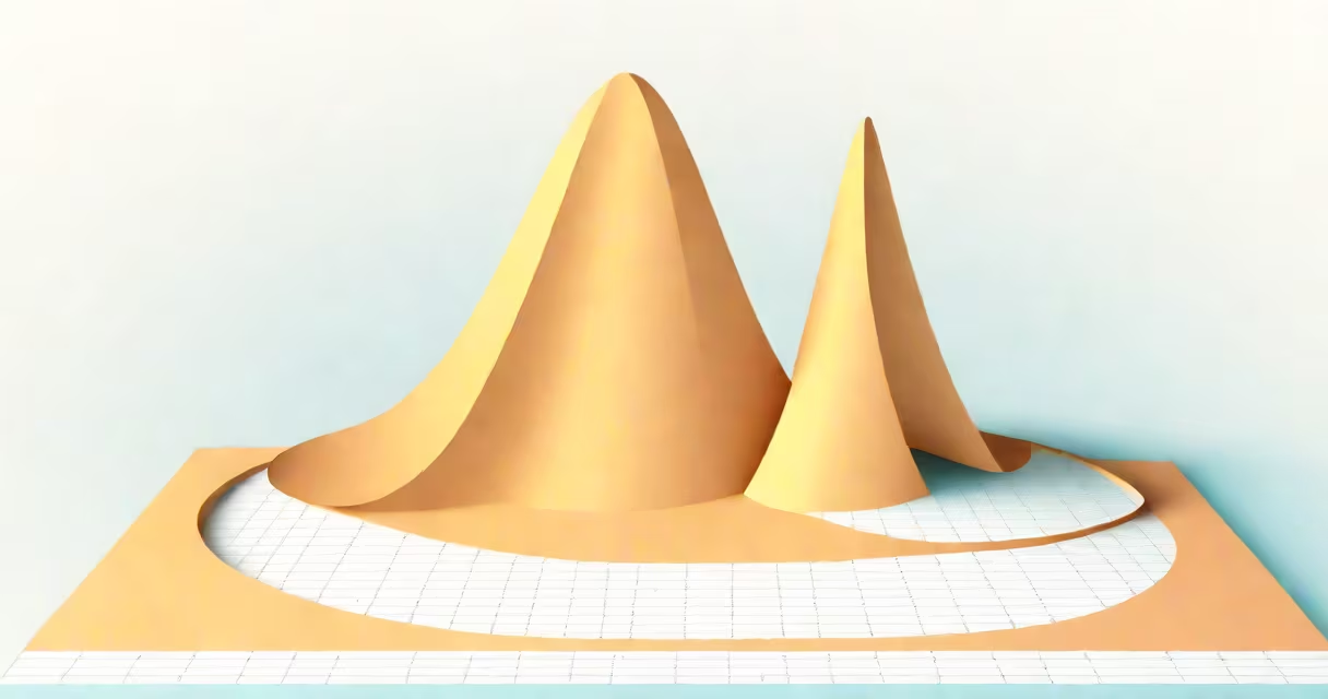
A normal curve graph, also called a bell curve, is a symmetrical graph that shows how data points distribute around a central mean, with most values clustering near the average and fewer appearing farther away. This probability density function is defined by its mean (center point) and standard deviation (spread).
The graph represents the normal distribution, a continuous probability distribution where about 68% of values fall within one standard deviation of the mean, 95% within two, and 99.7% within three. The equation for the normal curve is:
f(x) = (1 / (σ√(2π))) * e^(-(x-μ)² / (2σ²))
where μ is the mean, σ is the standard deviation, and e is Euler's number.
The normal curve has three key features:
The normal curve is widely used in statistics, finance, and natural sciences to model phenomena like test scores, stock returns, and measurement errors. For example, IQ scores follow a normal distribution with a mean of 100 and a standard deviation of 15.
Many confuse the normal curve with other distributions, such as the binomial or Poisson. Unlike these, the normal curve is continuous and symmetrical. Another mistake is assuming all real-world data fits a normal distribution-many do not, requiring transformations or alternative models.
Suppose a class of 100 students takes a test with an average score of 75 and a standard deviation of 5. The normal curve graph would show most scores between 70 and 80, with fewer scores as you move away from the mean. Using the 68-95-99.7 rule, about 68 students scored between 70 and 80, 95 between 65 and 85, and 99.7 between 60 and 90.
I once used a normal curve graph to analyze employee performance reviews. By plotting scores against the mean, I identified outliers and adjusted training programs accordingly. The graph's symmetry helped visualize where most employees fell relative to expectations.
For more on how graphs work, see how the F-1 score is plotted on a graph.